RubberWithInclusion

This example demonstrates the Finite Kinematics newton solver for a composite consisting of a compliant rubber-like material and a (near) rigid metal or ceramic-like material. The difference in elastic moduli is 10x. The low faces (xlo, ylo, zlo) are homogeneous dirichlet in the normal direction and naumann in the lateral directions. The three-dimensional test yields the following:

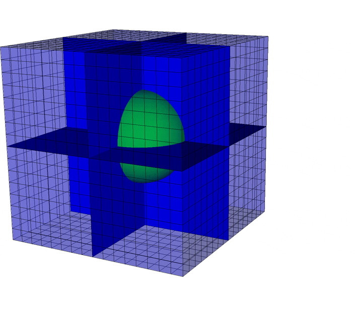
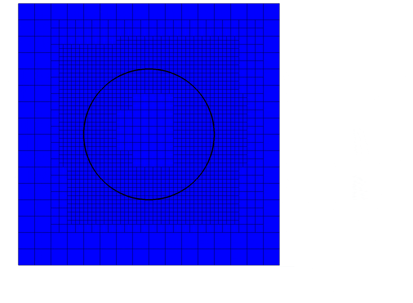
For regression testing purposes, only the two-dimensional case is considered for efficiency. In two dimensions, the distortion of the mesh is more severe, which usually means that additional Newton iterations are required.

[RubberWithInclusion] serial-2d

2d	Two-dimensional
square	Serial
verified	Testing script present
timer	13.8s (beaker)
play_circle	./bin/mechanics-2d-g++ tests/RubberWithInclusion/input

[RubberWithInclusion] serial-2d-coverage

2d	Two-dimensional
square	Serial
report_off	No testing script
play_circle	./bin/mechanics-2d-g++ tests/RubberWithInclusion/input stop_time="0.1"

[RubberWithInclusion] parallel-2d

2d	Two-dimensional
grid_view	Parallel (4 procs)
verified	Testing script present
timer	6.6s (beaker)
play_circle	mpiexec -np 4 ./bin/mechanics-2d-g++ tests/RubberWithInclusion/input

Input file (../../tests/RubberWithInclusion/input)

#@
#@ [serial-2d]
#@ exe=mechanics
#@ dim=2
#@ benchmark-beaker=13.8
#@ check-file=reference/thermo.dat
#@
#@ [serial-2d-coverage]
#@ exe=mechanics
#@ dim=2
#@ check=false
#@ args=stop_time=0.1
#@ coverage=true
#@
#@ [parallel-2d]
#@ exe=mechanics
#@ dim=2
#@ nprocs=4
#@ benchmark-beaker=6.6
#@ check-file=reference/thermo.dat
#@

alamo.program = mechanics
alamo.program.mechanics.model = finite.neohookean
plot_file = tests/RubberWithInclusion/output
type = static
timestep = 0.1
stop_time = 1.0

amr.plot_int = 1
amr.max_level = 2 
amr.n_cell = 16 16 16
amr.blocking_factor = 2
amr.thermo.int = 1
amr.thermo.plot_int = 1

geometry.prob_lo = 0 0 0
geometry.prob_hi = 1 1 1

ic.type = ellipse
ic.ellipse.a = 0.25 0.25 0.25
ic.ellipse.x0 = 0.5 0.5 0.5
ic.ellipse.eps = 0.05

nmodels = 2
model1.mu = 30
model1.kappa = 60
model2.mu = 3.0
model2.kappa = 6.0

solver.verbose = 3
solver.max_iter = 150
solver.nriters = 1000
solver.nrtolerance = 1E-5


ref_threshold = 100

bc.type = tension_test
bc.tension_test.type = uniaxial_stress
bc.tension_test.disp = (0,1:0,0.5)

solver.dump_on_fail = 1
amrex.signal_handling = 0
amrex.throw_exception = 1