Eshelby
This example demonstrates the Mechanics solver using the Eshelby inclusion problem. The example primarily tests the following Alamo capabilities
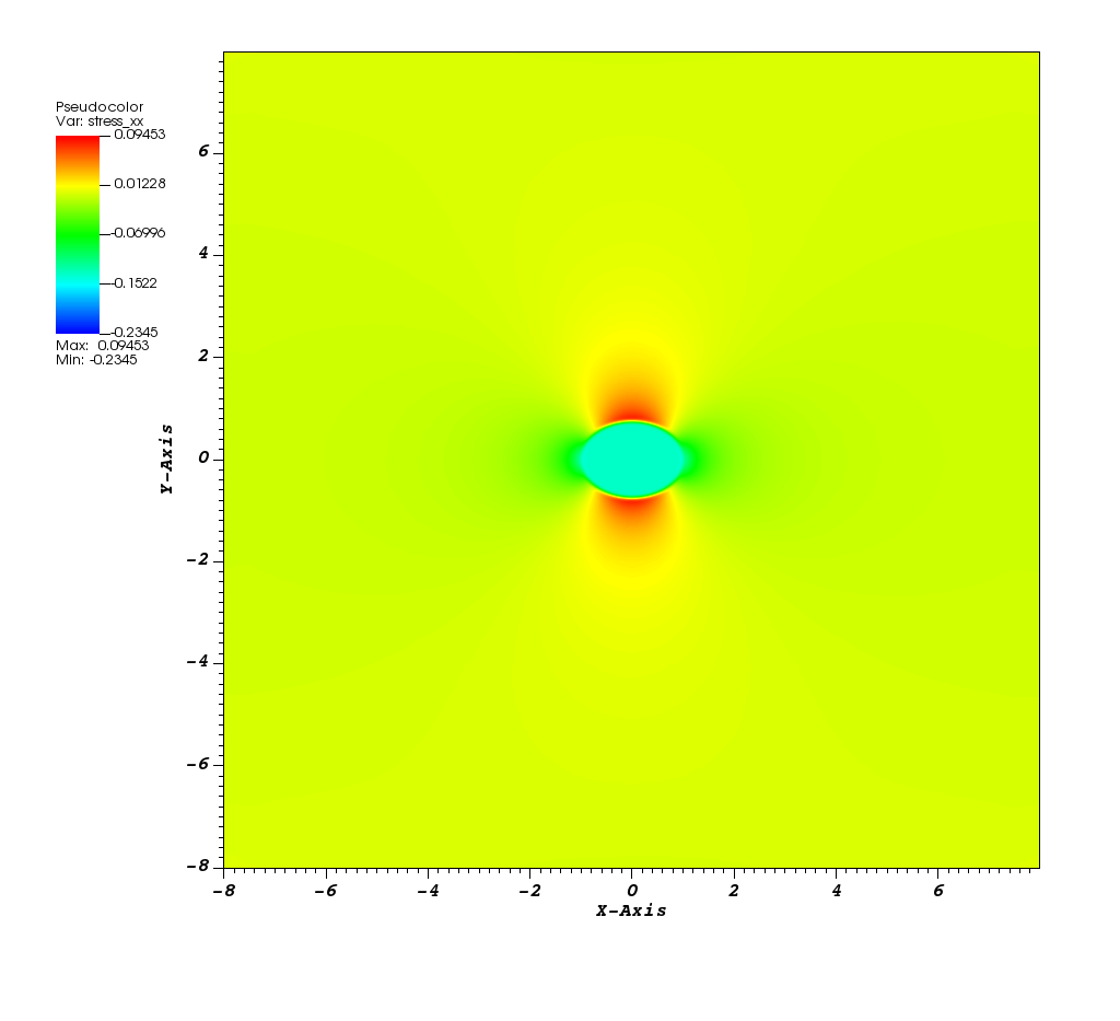
In 2D, the sigma_xx solution is:
In 3D, the solution is tested against the exact solution derived using Eshelby inclusion theory. For additional background see Runnels et al: https://doi.org/10.1016/j.jcp.2020.110065
2D-serial-5levels
Two-dimensional |
|
Serial |
|
Not validated |
|
./bin/mechanics-2d-g++ tests/Eshelby/input
|
2D-serial-5levels-coverage
Two-dimensional |
|
Serial |
|
Not validated |
|
./bin/mechanics-2d-g++ tests/Eshelby/input amr.max_level="3"
|
3D-serial-4levels
Three-dimensional |
|
Serial |
|
Validated using check script |
|
16.10s (beaker) 11.36s (statler) 22.75s (github) |
|
./bin/mechanics-3d-g++ tests/Eshelby/input amr.max_level="4"
|
3D-parallel-5levels
Three-dimensional |
|
Parallel (4 procs) |
|
Validated using check script |
|
24.66s (beaker) 18.76s (statler) |
|
mpiexec -np 4 ./bin/mechanics-3d-g++ tests/Eshelby/input
|
Input file (../../tests/Eshelby/input)
#@  [2D-serial-5levels]
#@  exe    = mechanics
#@  dim    = 2
#@  nprocs = 1
#@  check  = false
#@
#@  [2D-serial-5levels-coverage]
#@  exe    = mechanics
#@  dim    = 2
#@  nprocs = 1
#@  check  = false
#@  coverage = true
#@  args=amr.max_level=3
#@
#@  [3D-serial-4levels]
#@  exe    = mechanics
#@  dim    = 3
#@  nprocs = 1
#@  args   = amr.max_level=4
#@  benchmark-beaker = 16.10
#@  benchmark-statler = 11.36
#@  benchmark-github = 22.75
#@
#@  [3D-parallel-5levels]
#@  exe    = mechanics
#@  dim    = 3
#@  nprocs = 4
#@  benchmark-beaker = 24.66
#@  benchmark-statler = 18.76


alamo.program = mechanics
alamo.program.mechanics.model = affine.isotropic

plot_file		    = tests/Eshelby/output

# this is not a time integration, so do
# exactly one timestep and then quit
timestep		    = 0.1
stop_time		    = 0.1

# amr parameters
amr.plot_int		    = 1
amr.max_level		    = 5
amr.n_cell		    = 32 32 32
amr.blocking_factor	    = 8
amr.regrid_int		    = 1
amr.grid_eff		    = 1.0
amr.cell.all                = 1

# geometry
geometry.prob_lo	    = -8 -8 -8
geometry.prob_hi	    = 8 8 8
geometry.is_periodic	    = 0 0 0

# ellipse configuration
ic.type        = ellipse
ic.ellipse.a   = 1.0 0.75 0.5  # ellipse radii
ic.ellipse.x0  = 0 0 0 # location of ellipse center
ic.ellipse.eps = 0.1 # diffuse boundary

# elastic moduli
nmodels = 2
model1.E = 210
model1.nu = 0.3
model1.F0  = 0.001 0 0 0 0.001 0 0 0 0.001 # eigenstrain
model2.E = 210
model2.nu = 0.3
model2.F0  = 0 0 0 0 0 0 0 0 0 # eigenstrain

solver.verbose = 3
solver.nriters = 1
solver.max_iter = 20

bc.type = constant