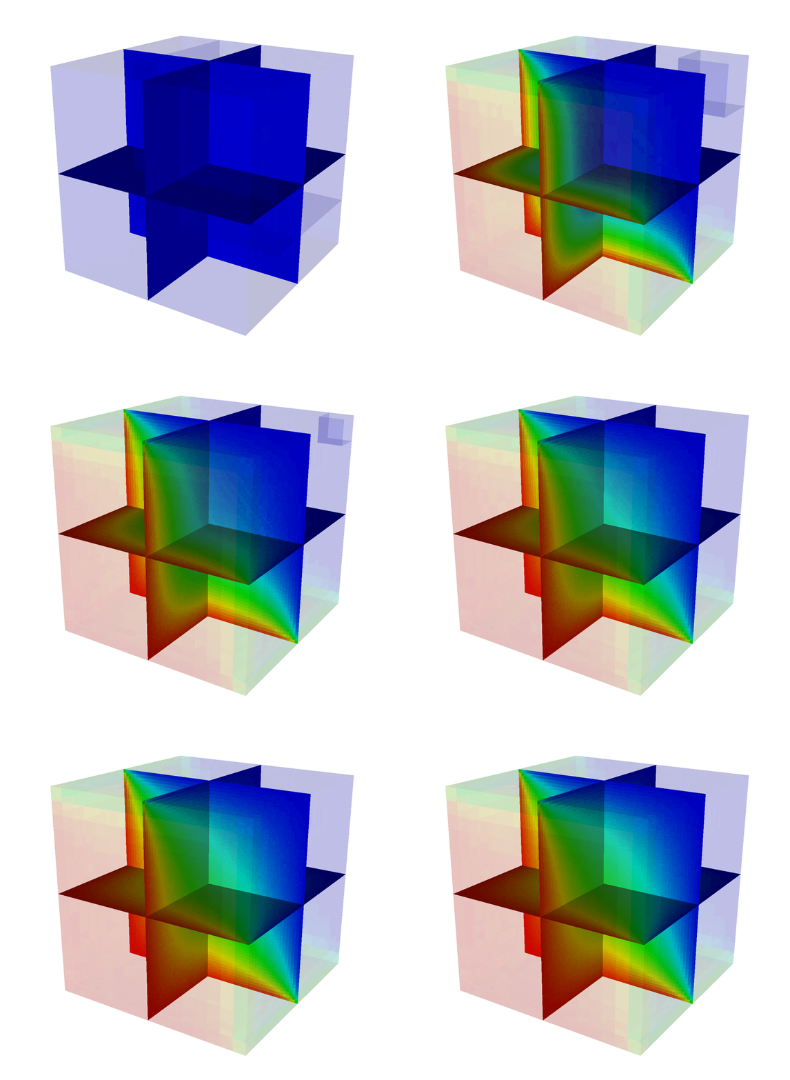
EshelbyDynamics
This test demonstrates the use of the dynamics solver using the Integrator::Mechanics integrator. It is similar to the Eshelby test problem: the inclusion is given an eigenstrain and compressed. This creates a stress wave at the interface into and out of the inclusion. Viscosity is used to damp out spurious oscillations, and so the solution converges fairly quickly to the static solution.

2D-serial-4levels
Two-dimensional |
|
Serial |
|
Validated using check script |
|
42s (beaker) |
|
./bin/mechanics-2d-g++ tests/EshelbyDynamics/input stop_time="0.5"
|
Input file (../../tests/EshelbyDynamics/input)
#@
#@  [2D-serial-4levels]
#@  exe    = mechanics
#@  dim    = 2
#@  nprocs = 1
#@  args   = stop_time=0.5
#@  check  = true
#@  benchmark-beaker = 42
#@

alamo.program = mechanics
alamo.program.mechanics.model = affine.isotropic

plot_file		    = tests/EshelbyDynamics/output

type=dynamic

# this is not a time integration, so do
# exactly one timestep and then quit
timestep		    = 0.0005
stop_time		    = 10.0

# amr parameters
amr.plot_dt		    = 0.01
amr.max_level		    = 4
amr.n_cell		    = 64 64 64
amr.blocking_factor	    = 8
amr.regrid_int		    = 100
amr.grid_eff		    = 1.0
amr.cell.all                = 1

# geometry
geometry.prob_lo	    = -8 -8 -8
geometry.prob_hi	    = 8 8 8
geometry.is_periodic	    = 0 0 0

# ellipse configuration
ic.type        = ellipse
ic.ellipse.a   = 1.0 0.75 0.5  # ellipse radii
ic.ellipse.x0  = 0 0 0 # location of ellipse center
ic.ellipse.eps = 0.1 # diffuse boundary

# elastic moduli
nmodels = 2
model1.E = 210
model1.nu = 0.3
model1.F0  = 0.001 0 0 0 0.001 0 0 0 0.001 # eigenstrain
model2.E = 210
model2.nu = 0.3
model2.F0  = 0 0 0 0 0 0 0 0 0 # eigenstrain

ref_threshold = 1000000000

viscous.mu_dashpot = 0.1
viscous.mu_newton  = 1.0

bc.type = constant